Coordinate Systems

In the last tutorial we learned how we can use matrices to our advantage by transforming all vertices with transformation matrices. OpenGL expects all the vertices, that we want to become visible, to be in normalized device coordinates after each vertex shader run. That is, the x, y and z coordinates of each vertex should be between -1.0 and 1.0; coordinates outside this range will not be visible. What we usually do, is specify the coordinates in a range we configure ourselves and in the vertex shader transform these coordinates to NDC. These NDC coordinates are then given to the rasterizer to transform them to 2D coordinates/pixels on your screen.

Transforming coordinates to NDC and then to screen coordinates is usually accomplished in a step-by-step fashion where we transform an object’s vertices to several coordinate systems before finally transforming them to screen coordinates. The advantage of transforming them to several intermediate coordinate systems is that some operations/calculations are easier in certain coordinate systems as will soon become apparent. There are a total of 5 different coordinate systems that are of importance to us:

• Local space (or Object space)
• World space
• View space (or Eye space)
• Clip space
• Screen space

Those are all a different state at which our vertices will be transformed in before finally ending up as fragments.

You’re probably quite confused by now by what a space or coordinate system actually is so we’ll explain them in a more understandable fashion by showing the total picture and what each specific space actually does.

The global picture

To transform the coordinates in one space to the next coordinate space we’ll use several transformation matrices of which the most important are the model, view and projection matrix. Our vertex coordinates first start in local space as local coordinates and are then further processed to world coordinates, Definition, view coordinatesclip coordinates and eventually end up as screen coordinates. The following image displays the process and shows what each transformation does:

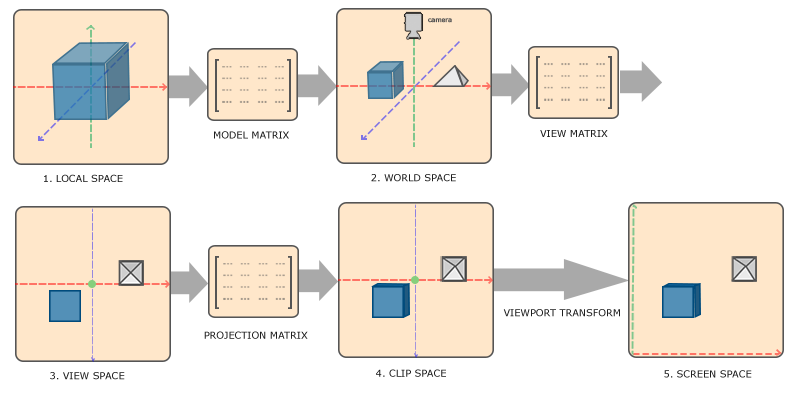
1. Local coordinates are the coordinates of your object relative to its local origin; they’re the coordinates your object begins in.
2. The next step is to transform the local coordinates to world-space coordinates which are coordinates in respect of a larger world. These coordinates are relative to a global origin of the world, together with many other objects also placed relative to the world’s origin.
3. Next we transform the world coordinates to view-space coordinates in such a way that each coordinate is as seen from the camera or viewer’s point of view.
4. After the coordinates are in view space we want to project them to clip coordinates. Clip coordinates are processed to the -1.0 and 1.0 range and determine which vertices will end up on the screen.
5. And lastly we transform the clip coordinates to screen coordinates in a process we call viewport transform that transforms the coordinates from -1.0 and 1.0 to the coordinate range defined by glViewport. The resulting coordinates are then sent to the rasterizer to turn them into fragments.

You probably got a slight idea what each individual space is used for. The reason we’re transforming our vertices into all these different spaces is that some operations make more sense or are easier to use in certain coordinate systems. For example, when modifying your object it makes most sense to do this in local space, while calculating certain operations on the object with respect to the position of other objects makes most sense in world coordinates and so on. If we want, we could define one transformation matrix that goes from local space to clip space all in one go, but that leaves us with less flexibility.

We’ll discuss each coordinate system in more detail below.

Local space

Local space is the coordinate space that is local to your object, i.e. where your object begins in. Imagine that you’ve created your cube in a modeling software package (like Blender). The origin of your cube is probably at (0,0,0) even though your cube might end up at a different location in your final application. Probably all the models you’ve created all have (0,0,0) as their initial position. All the vertices of your model are therefore in local space: they are all local to your object.

The vertices of the container we’ve been using were specified as coordinates between -0.5 and 0.5 with 0.0 as its origin. These are local coordinates.

World space

If we would import all our objects directly in the application they would probably all be somewhere stacked on each other around the world’s origin of (0,0,0) which is not what we want. We want to define a position for each object to position them inside a larger world. The coordinates in world space are exactly what they sound like: the coordinates of all your vertices relative to a (game) world. This is the coordinate space where you want your objects transformed to in such a way that they’re all scattered around the place (preferably in a realistic fashion). The coordinates of your object are transformed from local to world space; this is accomplished with the model matrix.

The model matrix is a transformation matrix that translates, scales and/or rotates your object to place it in the world at a location/orientation they belong to. Think of it as transforming a house by scaling it down (it was a bit too large in local space), translating it to a suburbia town and rotating it a bit to the left on the y-axis so that it neatly fits with the neighboring houses. You could think of the matrix in the previous tutorial to position the container all over the scene as a sort of model matrix as well; we transformed the local coordinates of the container to some different place in the scene/world.

View space

The view space is what people usually refer to as the camera of OpenGL (it is sometimes also known as the camera space or eye space). The view space is the result of transforming your world-space coordinates to coordinates that are in front of the user’s view. The view space is thus the space as seen from the camera’s point of view. This is usually accomplished with a combination of translations and rotations to translate/rotate the scene so that certain items are transformed to the front of the camera. These combined transformations are generally stored inside a view matrix that transforms world coordinates to view space. In the next tutorial we’ll extensively discuss how to create such a view matrix to simulate a camera.

Clip space

At the end of each vertex shader run, OpenGL expects the coordinates to be within a specific range and any coordinate that falls outside this range is clipped. Coordinates that are clipped are discarded, so the remaining coordinates will end up as fragments visible on your screen. This is also where clip space gets its name from.

Because specifying all the visible coordinates to be within the range -1.0 and 1.0 isn’t really intuitive, we specify our own coordinate set to work in and convert those back to NDC as OpenGL expects them.

To transform vertex coordinates from view to clip-space we define a so called projection matrix that specifies a range of coordinates e.g. -1000 and 1000 in each dimension. The projection matrix then transforms coordinates within this specified range to normalized device coordinates (-1.0, 1.0). All coordinates outside this range will not be mapped between -1.0 and 1.0 and therefore be clipped. With this range we specified in the projection matrix, a coordinate of (1250, 500, 750) would not be visible, since the x coordinate is out of range and thus gets converted to a coordinate higher than 1.0 in NDC and is therefore clipped.

Note that if only a part of a primitive e.g. a triangle is outside the clipping volume OpenGL will reconstruct the triangle as one or more triangles to fit inside the clipping range.

This viewing box a projection matrix creates is called a frustum and each coordinate that ends up inside this frustum will end up on the user’s screen. The total process to convert coordinates within a specified range to NDC that can easily be mapped to 2D view-space coordinates is called projection since the projection matrix projects 3D coordinates to the easy-to-map-to-2D normalized device coordinates.

Once all the vertices are transformed to clip space a final operation called perspective division is performed where we divide the x, y and z components of the position vectors by the vector’s homogeneous w component; perspective division is what transforms the 4D clip space coordinates to 3D normalized device coordinates. This step is performed automatically at the end of each vertex shader run.

It is after this stage where the resulting coordinates are mapped to screen coordinates (using the settings of glViewport) and turned into fragments.

The projection matrix to transform view coordinates to clip coordinates can take two different forms, where each form defines its own unique frustum. We can either create an orthographic projection matrix or a perspective projection matrix.

Orthographic projection

An orthographic projection matrix defines a cube-like frustum box that defines the clipping space where each vertex outside this box is clipped. When creating an orthographic projection matrix we specify the width, height and length of the visible frustum. All the coordinates that end up inside this frustum after transforming them to clip space with the orthographic projection matrix won’t be clipped. The frustum looks a bit like a container:

The frustum defines the visible coordinates and is specified by a width, a height and a near and far plane. Any coordinate in front of the near plane is clipped and the same applies to coordinates behind the far plane. The orthographic frustum directly maps all coordinates inside the frustum to normalized device coordinates since the w component of each vector is untouched; if the w component is equal to 1.0 perspective division doesn’t change the coordinates.

To create an orthographic projection matrix we make use of SGLMath’s function ortho:

let projection:mat4 = SGLMath.ortho(0.0, 800.0, 0.0, 600.0, 0.1, 100.0)

The first two parameters specify the left and right coordinate of the frustum and the third and fourth parameter specify the bottom and top part of the frustum. With those 4 points we’ve defined the size of the near and far planes and the 5th and 6th parameter then define the distances between the near and far plane. This specific projection matrix transforms all coordinates between these x, y and z range values to normalized device coordinates.

An orthographic projection matrix directly maps coordinates to the 2D plane that is your screen, but in reality a direct projection produces unrealistic results since the projection doesn’t take perspective into account. That is something the perspective projection matrix fixes for us.

Perspective projection

If you ever were to enjoy the graphics the real life has to offer you’ll notice that objects that are farther away appear much smaller. This weird effect is something we call perspective. Perspective is especially noticeable when looking down the end of an infinite motorway or railway as seen in the following image:

As you can see, due to perspective the lines seem to coincide the farther they’re away. This is exactly the effect perspective projection tries to mimic and it does so using a perspective projection matrix. The projection matrix maps a given frustum range to clip space, but also manipulates the w value of each vertex coordinate in such a way that the further away a vertex coordinate is from the viewer, the higher this w component becomes. Once the coordinates are transformed to clip space they are in the range -w to w (anything outside this range is clipped). OpenGL requires that the visible coordinates fall between the range -1.0 and 1.0 as the final vertex shader output, thus once the coordinates are in clip space, perspective division is applied to the clip space coordinates:

Each component of the vertex coordinate is divided by its w component giving smaller vertex coordinates the further away a vertex is from the viewer. This is another reason why the w component is important, since it helps us with perspective projection. The resulting coordinates are then in normalized device space. If you’re interested to figure out how the orthographic and perspective projection matrices are actually calculated (and aren’t too scared of mathematics) I can recommend this excellent article by Songho.

A perspective projection matrix can be created in SGLMath as follows:

let proj:mat4 = SGLMath.perspective(radians(45.0), Float(width)/Float(height), 0.1, 100.0)

What SGLMath.perspective does is again create a large frustum that defines the visible space, anything outside the frustum will not end up in the clip space volume and will thus become clipped. A perspective frustum can be visualized as a non-uniformly shaped box from where each coordinate inside this box will be mapped to a point in clip space. An image of a perspective frustum is seen below:

Its first parameter defines the fov value, that stands for field of view and sets how large the viewspace is. For a realistic view it is usually set at 45.0f, but for more doom-style results you could set it to a higher value. The second parameter sets the aspect ratio which is calculated by dividing the viewport’s width by its height. The third and fourth parameter set the near and far plane of the frustum. We usually set the near distance to 0.1f and the far distance to 100.0f. All the vertices between the near and far plane and inside the frustum will be rendered.

Whenever the near value of your perspective matrix is set a bit too high (like 10.0f), OpenGL will clip all coordinates close to the camera (between 0.0f and 10.0f), which gives a familiar visual result in videogames in that you can see through certain objects if you move too close to them.

When using orthographic projection, each of the vertex coordinates are directly mapped to clip space without any fancy perspective division (it still does perspective division, but the w component is not manipulated (it stays 1) and thus has no effect). Because the orthographic projection doesn’t use perspective projection, objects farther away do not seem smaller, which produces a weird visual output. For this reason the orthographic projection is mainly used for 2D renderings and for some architectural or engineering applications where we’d rather not have vertices distorted by perspective. Applications like Blender that are used for 3D modelling sometimes use orthographic projection for modelling, because it more accurately depicts each object’s dimensions. Below you’ll see a comparison of both projection methods in Blender:

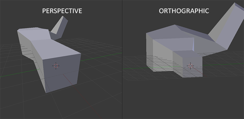
You can see that with perspective projection, the vertices farther away appear much smaller, while in orthographic projection each vertex has the same distance to the user.

Putting it all together

We create a transformation matrix for each of the aforementioned steps: model, view and projection matrix. A vertex coordinate is then transformed to clip coordinates as follows:

Note that the order of matrix multiplication is reversed (remember that we need to read matrix multiplication from right to left). The resulting vertex should then be assigned to gl_Position in the vertex shader and OpenGL will then automatically perform perspective division and clipping.

And then?
The output of the vertex shader requires the coordinates to be in clip-space which is what we just did with the transformation matrices. OpenGL then performs perspective division on the clip-space coordinates to transform them to normalized-device coordinates. OpenGL then uses the parameters from glViewPort to map the normalized-device coordinates to screen coordinates where each coordinate corresponds to a point on your screen (in our case a 800x600 screen). This process is called the viewport transform.

This is a difficult topic to understand so if you’re still not exactly sure about what each space is used for you don’t have to worry. Below you’ll see how we can actually put these coordinate spaces to good use and enough examples will follow in these tutorials.

Going 3D

Now that we know how to transform 3D coordinates to 2D coordinates we can start showing our objects as real 3D objects instead of a lame 2D plane we’ve been showing so far.

To start drawing in 3D we’ll first create a model matrix. The model matrix consists of translations, scaling and/or rotations we’d like to apply to transform all object’s vertices it to the global world space. Let’s transform our plane a bit by rotating it on the x-axis so the top is further away than the bottom. The model matrix then looks like this:

var model = SGLMath.rotate(mat4(), radians(-55.0), vec3(1.0, 0.0, 0.0))

By multiplying the vertex coordinates with this model matrix we’re transforming the vertex coordinates to world coordinates. Our plane that is tipped away from us thus represents the plane in the global world.

Next we need to create a view matrix. We want to move slightly backwards in the scene so the object becomes visible (when in world space we’re located at the origin (0,0,0)). To move around the scene, think about the following:

• To move a camera backwards, is the same as moving the entire scene forward.

That is exactly what a view matrix does, we move the entire scene around inversed to where we want the camera to move. Because we want to move backwards and since OpenGL is a right-handed system we have to move in the positive z-axis. We do this by translating the scene towards the negative z-axis. This gives the impression that we are moving backwards.

We’ll discuss how to move around the scene in more detail in the next tutorial. For now the view matrix looks like this:

// Translating the scene away from us has the
// same effect as stepping back from the scene
var view = SGLMath.translate(mat4(), vec3(0.0, 0.0, -3.0))

The last thing we need to define is the projection matrix. We want to use perspective projection for our scene so we’ll declare the projection matrix like this:

let aspectRatio = GLfloat(WIDTH) / GLfloat(HEIGHT)
var projection = SGLMath.perspective(radians(45.0), aspectRatio, 0.1, 100.0)

Now that we created the transformation matrices we should pass them to our shaders. First let’s declare the transformation matrices as uniforms in the vertex shader and multiply them with the vertex coordinates.

#version 330 core
layout (location = 0) in vec3 position;
layout (location = 1) in vec2 texCoord;

out vec2 TexCoord;
  
uniform mat4 model;
uniform mat4 view;
uniform mat4 projection;

void main()
{
    gl_Position = projection * view * model * vec4(position, 1.0f);
    TexCoord = texCoord;
}

We should also send the matrices to the shader (this is usually done each render iteration since transformation matrices tend to change a lot):

let modelLoc = glGetUniformLocation(ourShader.program, "model")
withUnsafePointer(&model, {
    glUniformMatrix4fv(modelLoc, 1, false, UnsafePointer($0))
})
// ... repeat for view and projection matrices

Now that our vertex coordinates are transformed via the model, view and projection matrix the final object should be:

• Tilted backwards to the floor.
• A bit farther away from us.
• Be displayed with perspective.

Let’s check if the result actually does fulfill these requirements:

It does indeed look like the plane is a 3D plane that’s falling away towards the floor. If you’re not getting the same result check the complete source code.

More 3D

So far we’ve been working with a 2D plane, even in 3D space, so let’s take the adventurous route and extend our 2D plane to a 3D cube. To render a cube we need a total of 36 vertices (6 faces * 2 triangles * 3 vertices each). 36 vertices are a lot to sum up so you can retrieve them from here. Note that we’re omitting the color values, since we’ll only be using textures to get the final color value.

For fun, we’ll let the cube rotate over time:

var model = SGLMath.rotate(mat4(), GLfloat(glfwGetTime()), vec3(0.5, 1.0, 0.0))

And then we’ll draw the cube using glDrawArrays, but this time with a count of 36 vertices.

glDrawArrays(GL_TRIANGLES, 0, 36)

You should get something similar to the following:

It does resemble a cube slightly but something’s off. Some sides of the cubes are being drawn over other sides of the cube. This happens because when OpenGL draws your cube triangle-by-triangle, it will overwrite its pixels even though something else might’ve been drawn there before. Because of this, some triangles are drawn on top of each other while they’re not supposed to overlap.

Luckily, OpenGL stores depth information in a buffer called the z-buffer that allows OpenGL to decide when to draw over a pixel and when not to. Using the z-buffer we can configure OpenGL to do depth-testing.

Z-buffer

OpenGL stores all its depth information in a z-buffer, also known as a depth buffer. GLFW automatically creates such a buffer for you (just like it has a color-buffer that stores the colors of the output image). The depth is stored within each fragment (as the fragment’s z value) and whenever the fragment wants to output its color, OpenGL compares its depth values with the z-buffer and if the current fragment is behind the other fragment it is discarded, otherwise overwritten. This process is called depth testing and is done automatically by OpenGL.

However, if we want to make sure OpenGL actually performs the depth testing we first need to tell OpenGL we want to enable depth testing; it is disabled by default. We can enable depth testing using glEnable. The glEnable and glDisable functions allow us to enable/disable certain functionality in OpenGL. That functionality is then enabled/disabled until another call is made to disable/enable it. Right now we want to enable depth testing by enabling GL_DEPTH_TEST:

glEnable(GL_DEPTH_TEST)

Since we’re using a depth buffer we also want to clear the depth buffer before each render iteration (otherwise the depth information of the previous frame stays in the buffer). Just like clearing the color buffer, we can clear the depth buffer by specifying the DEPTH_BUFFER_BIT bit in the glClear function:

glClear(GL_COLOR_BUFFER_BIT | GL_DEPTH_BUFFER_BIT)

Let’s re-run our program and see if OpenGL now performs depth testing:

There we go! A fully textured cube with proper depth testing that rotates over time. Check the source code here.

More cubes!

Say we wanted to display 10 of our cubes on screen. Each cube will look the same but will only differ in where it’s located in the world with each a different rotation. The graphical layout of the cube is already defined so we don’t have to change our buffers or attribute arrays when rendering more objects. The only thing we have to change for each object is its model matrix where we transform the cubes into the world.

First, let’s define a translation vector for each cube that specifies its position in world space. We’ll define 10 cube positions in a vec3 array:

let cubePositions:[vec3] = [
  [ 0.0,  0.0,  0.0], 
  [ 2.0,  5.0, -15.0], 
  [-1.5, -2.2, -2.5],  
  [-3.8, -2.0, -12.3],  
  [ 2.4, -0.4, -3.5],  
  [-1.7,  3.0, -7.5],  
  [ 1.3, -2.0, -2.5],  
  [ 1.5,  2.0, -2.5], 
  [ 1.5,  0.2, -1.5], 
  [-1.3,  1.0, -1.5]  
]   

Now, within the game loop we want to call the glDrawArrays function 10 times, but this time send a different model matrix to the vertex shader each time before we render. We will create a small loop within the game loop that renders our object 10 times with a different model matrix. Note that we also add a small rotation to each container.

glBindVertexArray(VAO)
let modelLoc = glGetUniformLocation(ourShader.program, "model")
for (index, cubePosition) in cubePositions.enumerate() {
  var model = mat4()
  model = SGLMath.translate(model, cubePosition)
  model = SGLMath.rotate(model, Float(index), vec3(0.5, 1.0, 0.0))
  withUnsafePointer(&model, {
      glUniformMatrix4fv(modelLoc, 1, false, UnsafePointer($0))
  })
  glDrawArrays(GL_TRIANGLES, 0, 36)
}
glBindVertexArray(0)

This snippet of code will update the model matrix each time a new cube is drawn and do this 10 times in total. Right now we should be looking into a world filled with 10 oddly rotated cubes:

Perfect! It looks like our container found some likeminded friends. If you’re stuck see if you can compare your code with the source code.

Exercises

• Try experimenting with the FoV and aspect-ratio parameters of SGLMath’s projection function. See if you can figure out how those affect the perspective frustum.
• Play with the view matrix by translating in several directions and see how the scene changes. Think of the view matrix as a camera object.
• Try to make every 3rd container (including the 1st) rotate over time, while leaving the other containers static using just the model matrix.